
The easiest way to treat sequential data would be simply to ignore the sequential aspects and treat the observations as independent and identically distributed (i.i.d.)[Bishop 2006] as shown in Figure 1. However, this approach would fail to exploit sequential patterns. It is possible to measure relative frequency, but for next state prediction, it would be significant help to observe patterns in near past with their correlations with each other.
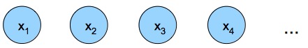
Figure 1: simplest approach to modeling a sequence of observations
To express correlation effect in such probabilistic model, relaxation takes place, considering Markov Model. Joint distribution for particular sequence of observations can be express the product rules in the form
p(x1,…,xN) = Π(n=1; N) p(xn | x1,…,xn-1 )
In case each of the conditional distributions is only dependent on most recent observation, it is called first-order Markov chain, which is illustrated below.

Figure 2: first-order Markov chain
p(x1,…,xN) = p(x1) Π(n=2; N) p(xn | xn-1 )
This model, however does not allow one value, to be influenced by other than the one before. In order to allow such influence within model, it must be moved to higher-order Markov chain. Model, where new value is predicted from last two is called second-order Markov chain.

Figure 3: second-order Markov chain
p(x1,…,xN) = p(x1) Π(n=2; N) p(xn | xn-1 , xn-2)
Similarly we can consider extensions to Mth order Markov chain, where next state is dependent on previous M states. By this improvement in flexibility, we have paid by increasing the number of parameters.[Bishop 2006]
Hidden Markov Models
With this statistical Markov Model, one can model Markov process with unobserved states, also called “hidden states”. In this model, visible is only the output that is directly dependent on the invisible state. Each state is defined with probability distribution over possible outputs. Therefore generated sequence of outputs (or also called observations) can offer some information about state sequence, which is hidden. Everything except current or past states is known and can be used directly.
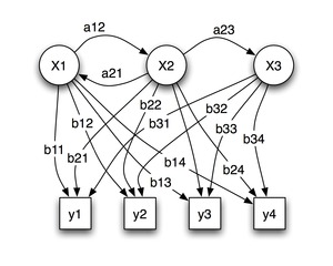
Figure 4: Example of Hidden Markov Model (Image source wikipedia.org)
-
Nodes labeled “x” are hidden states
-
“y” are observations
-
Arrows labeled “a” are state transition probabilities
-
Probability distribution over observations are labeled “b”
For better understanding of Hidden Markov Models, L. Rabiner in [Rabiner 1989] proposes The Urn and Ball Model: There are N glass urns with many colored balls inside. Balls can be colored with M distinct colors. Process of obtaining observations is maintained by genie. He chooses an urn by random, takes any ball and present the color. Then the ball is replaced in it’s urn. Next urn is then chosen according to the random selection process associated with the current urn. Another ball is chosen and presented. The whole process generates a finite observation sequence of colors. This is considered as observable output of a Hidden Markov Model. Sequence from which were balls chosen is not known. These are the hidden states. Choosing the next urn was organized by state transition probabilities and taking the specific ball from urn was managed by observation probability distribution. It could be influenced by amount of balls with specific color within the urn.
To connect this example with Figure 4, graph is the room with genie (abstract character representing the probability matrices) and three urns x1, x2, x3. There are four colors y1, y2, y3 and y4. Genie could have presented sequence of colors (observations) such as y2,y4,y1,y2,y2,y3,y1,y4,y1,y4 (example) in this order, but the sequence of urns (states) from where were these balls taken is not known. This information can be however calculated from sequence of observations and probability matrices for example with Viterbi algorithm.[Bishop 2006]
Bibliography
Bishop 2006: Christopher M. Bishop, Pattern recognition and machine learning, 2006
Rabiner 1989: Lawrence R. Rabiner, A Tutorial on Hidden Markov Models and Selected Applications in Speech Recognition, 1989
Facebook Comments
Hidden Markov Models